Update: Ported the code to Clojure too.

TL;DR: Inspired by a couple of posts implementing particle swarm optimization in Python and R, I implemented one in Guile Scheme. Here’s the Guile code, and here’s the Python translation of the same approach.

An approachable introduction to particle swarm optimization was published recently. Later I came across another post inspired from that one which used R.

Since I was playing with Scheme, I decided to port the algorithm to Guile. And while doing it, I have also changed how the code is organized. The Numpy and R versions use vectorized operations heavily, while I am modeling the domain using native data structures. This would probably have a slight performance cost but the code might be more understandable. (The Guile code itself might seem less understandable if Lisp-like languages aren’t familiar, but here’s an equivalent pure Python implementation for comparison.)

How it works

I will try to give an intuition of the algorithm by comparing it to gradient descent. For the formal description and equations check out the articles linked above.

Gradient descent is often described in terms of a blindfolded person finding the lowest point of a hilly landscape by taking steps in the direction of steepest descent till the bottom is reached. This only works if the derivative can be calculated at every step, and the searcher can also get stuck in a local valley, not knowing that a deeper valley exists. Different ways of taking the steps have been developed to increase chances of finding the deepest valley, but the image of this single person, quite possibly abducted, blundering his way blindfolded is not a happy one.

It might be better, not to mention more cheerful, to have a search party instead. This is the idea of swarms: A search party is organized and parachuted down on to the landscape. Each of them keeps track of wherever they have been and are in constant touch with everyone else. They know the best position they have personally seen, and the best position of the party. Each one moves by combining these pieces of information, and eventually converge somewhere close to the deepest point which they sought (where presumably a blindfolded body lies). No gradients necessary.

Imports and Utilities

Before we begin, here are two helper functions which add/subtract all the given vectors element-wise.

(use-modules (srfi srfi-1))

(define (vec-sub v1 v2 . ...)
  (map (lambda (xs) (apply - xs))
        (apply zip `(,v1 ,v2 ,@...))))

(define (vec-add v1 v2 . ...)
  (map (lambda (xs) (apply + xs))
        (apply zip `(,v1 ,v2 ,@...))))

(vec-add '(5 5) '(2 2)) ; => (7 7)
(vec-sub '(5 5) '(2 2)) ; => (3 3)

Making a Swarm

We will represent a swarm as a list of particles in the search space we define. A particle is modeled as an association list which holds its position, velocity, the best position it has seen so far, and the history of all the positions it has been at.

(define (make-particle xlims ylims)
  (let* ((xlo (first xlims))
         (xhi (second xlims))
         (ylo (first ylims))
         (yhi (second ylims))
         (coords (list (+ xlo (random (- xhi xlo))) (+ ylo (random (- yhi ylo)))))
         (velocity (list (* 0.1 (random 1.0)) (* 0.1 (random 1.0)))))
    (list (cons 'position coords)
          (cons 'best coords)
          (cons 'velocity velocity)
          (cons 'history (list coords)))))

(define (make-swarm xlims ylims nparticles)
  (let lp [(i 0)
           (res '())]
    (if (= i nparticles)
        res
        (lp (+ 1 i) (cons (make-particle xlims ylims) res)))))

Updating the Swarm

While each particle has the information about their personal best position, we write a function to get the best particle of a swarm to use in the update procedure.

(define (best-particle f swarm)
  (fold (lambda (p1 p2)
    (if (< (apply f (assoc-ref p1 'position))
           (apply f (assoc-ref p2 'position)))
        p1 p2))
  (car swarm)
  (cdr swarm)))

(define (update-swarm swarm f cognition cohesion inertia)
  (let [(global-best (best-particle f swarm))]
    (define (update-particle p)
      (let* [(v (assoc-ref p 'velocity))
             (xy (assoc-ref p 'position))
             (b (assoc-ref p 'best))
             (h (assoc-ref p 'history))
             (new-v (vec-add (map (lambda (x) (* x inertia)) v)
                             (map (lambda (x) (* x cognition (random 1.0)))
                                (vec-sub b xy))
                             (map (lambda (x) (* x cohesion (random 1.0)))
                                (vec-sub (assoc-ref global-best 'position) xy))))
             (new-xy (vec-add xy new-v))
             (new-h (cons new-xy h))
             (new-b (if (< (apply f new-xy) (apply f b)) new-xy b))]
    (list (cons 'velocity new-v)
          (cons 'position new-xy)
          (cons 'history new-h)
          (cons 'best new-b))))
    (map (lambda (p) (update-particle p)) swarm)))

Particle Swarm Optimization

At this point we have everything we need. We can pack it into a pso function which iteratively applies the update function on the swarm.

(define (pso f xlims ylims nparticles cognition cohesion inertia niter)
  (let lp [(i 0)
           (swarm (make-swarm xlims ylims nparticles))]
    (if (= i niter)
        (assoc-ref (best-particle f swarm) 'best)
        (lp (+ i 1) (update-swarm swarm f cognition cohesion inertia)))))

Running

I have ported the functions used in both the articles linked to at the top.

(define (mlmfunc x y)
  (+ (expt (- x 3.14) 2)
     (expt (- y 2.72) 2)
     (sin (+ (* 3 x) 1.41))
     (sin (- (* 4 y) 1.73))))

(define (ackley x y)
  (+ (- (* -20 (exp (* -0.2 (sqrt (* 0.5 (+ (expt (- x 1) 2) (expt (- y 1) 2)))))))
        (exp (* 0.5 (+ (cos (* 2 3.141592 x)) (cos (* 2 3.141592 y))))))
     (exp 1)
     20))

(pso mlmfunc '(0 5.) '(0 5.) 20 0.01 0.05 0.5 100)
(pso ackley '(-10 10.) '(-10 10.) 20 0.01 0.05 0.5 100)

This code seems to do what it’s supposed to and gives results that match the originals.

Extras: Getting data out

We can transfer the path histories of the particles into R to do visualizations. For this, instead of just returning the best position we make the function return the full swarm and then extract the position histories of the particles into a CSV.

(define (pso-full-swarm f xlims ylims nparticles cognition cohesion w niter)
  (let lp [(i 0)
           (swarm (make-swarm xlims ylims nparticles))]
    (if (= i niter)
        swarm
        (lp (+ i 1) (update-swarm swarm f cognition cohesion w)))))

(define (create-output-data output)
  (let* [(histories (map (lambda (p) (reverse (assoc-ref p 'history))) output))
         (zipped (apply zip histories))
         (steps-data (
           map (lambda (step)
                (map (lambda (xy) (cons (number->string step)
                                  (map number->string xy)))
                     (list-ref zipped step)))
                (iota (length zipped))))]
    (fold append (car steps-data) (cdr steps-data))))

(use-modules (csv csv))

(call-with-output-file "out.csv"
  (lambda (port)
    (sxml->csv 
      (create-output-data
        (pso-full-swarm mlmfunc '(0 5.) '(0 5.) 20 0.01 0.05 0.5 50))
      port)))

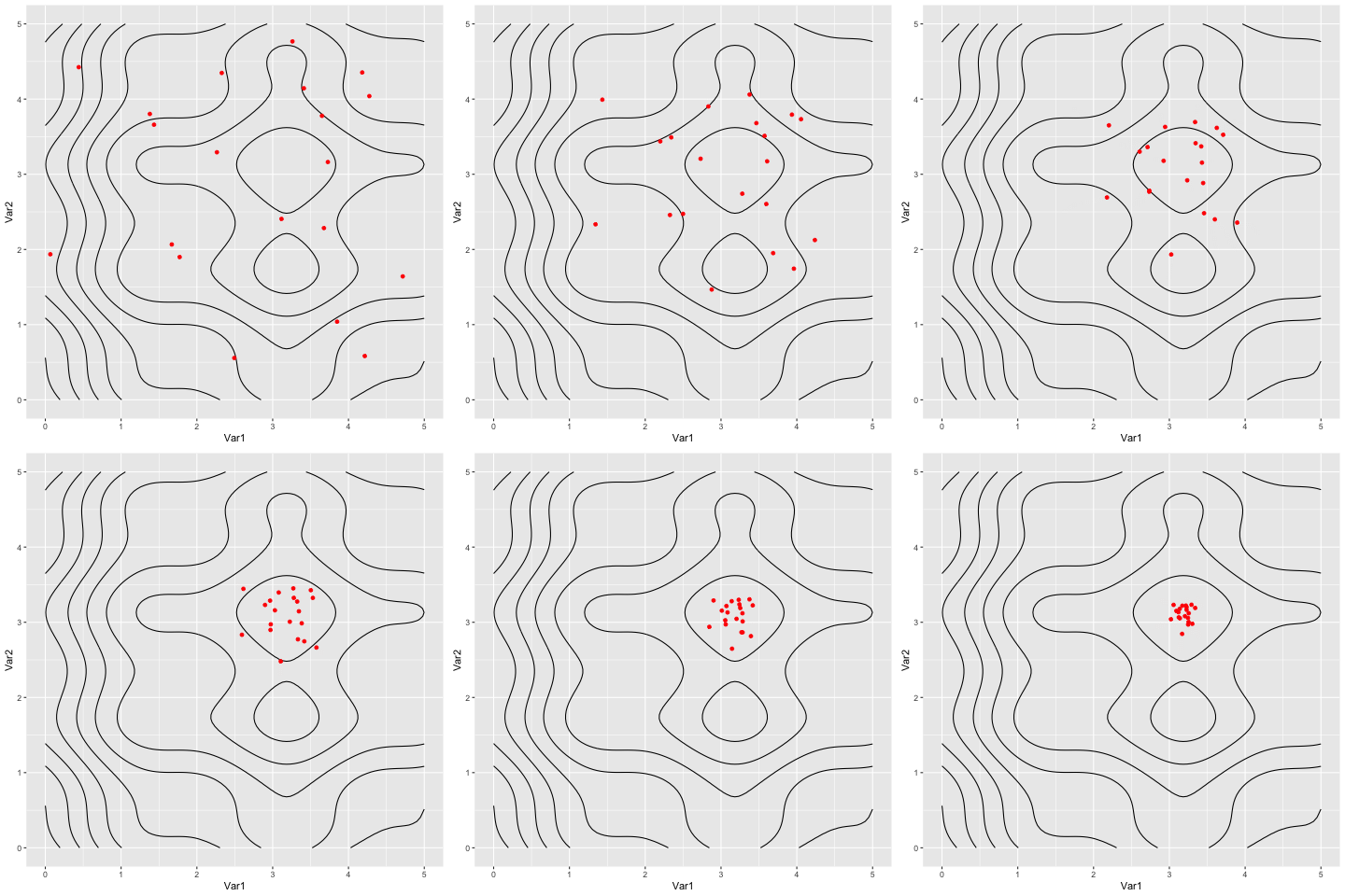
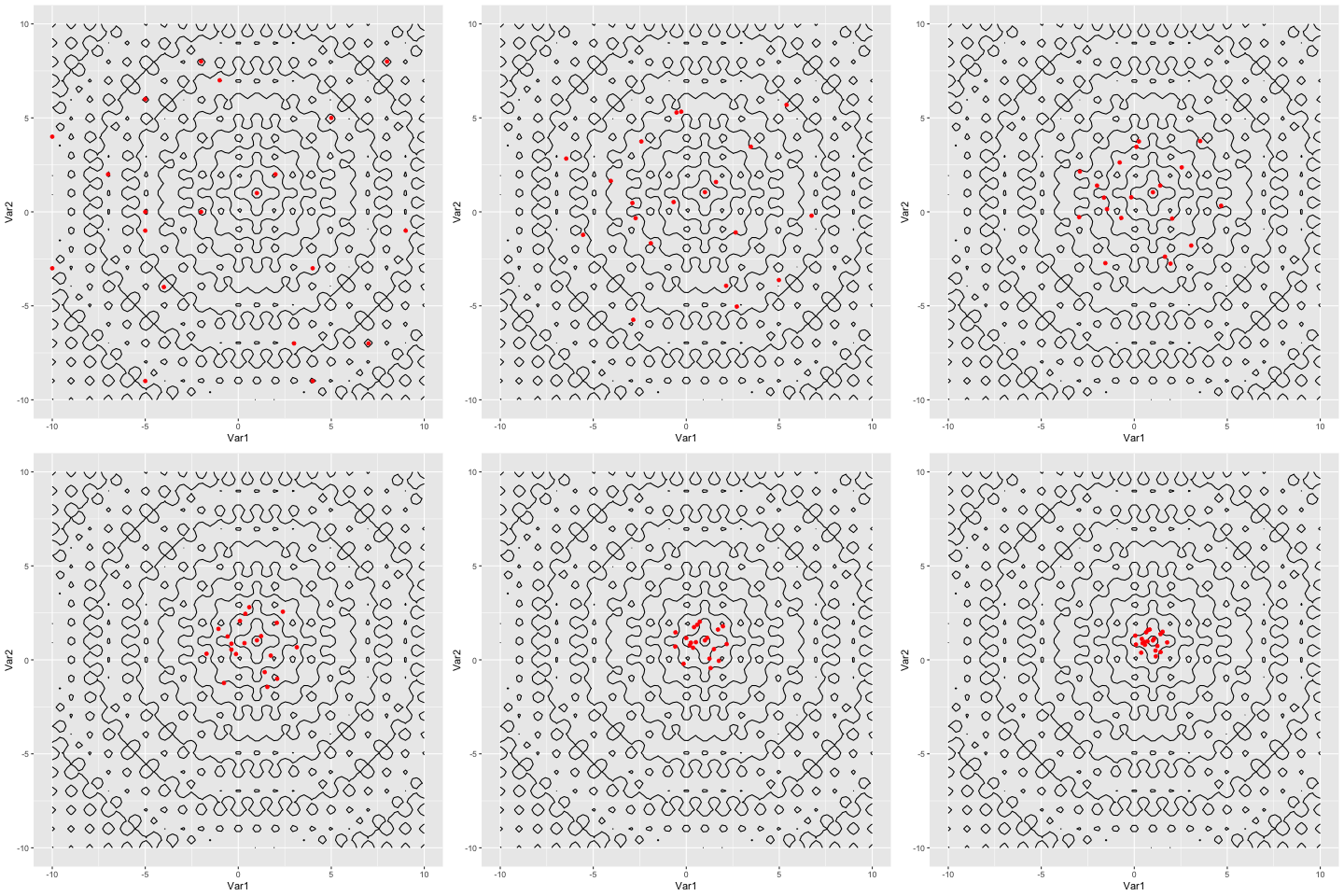
Once we have a CSV, we read it in to R, and make an animation of the particles converging.

library(tidyverse)
library(gganimate)

d <- read_csv("out.csv", col_names = c('step', 'x', 'y'))

f <- function(x, y) {
  (x - 3.14) ** 2 + (y - 2.72) ** 2 + sin(3 * x + 1.41) + sin(4 * y - 1.73)
}

x <- seq(0, 5, length.out = 100)
y <- seq(0, 5, length.out = 100)
grid <- expand.grid(x, y, stringsAsFactors = F)
grid$z <- f(grid[,1], grid[,2])

library(gganimate)

ggplot(d) +
  geom_contour(data = grid, aes(x = Var1, y = Var2, z = z), color = "black") +
  geom_point(aes(x, y), color = "red") +
  transition_states(step, state_length = .05)

Animations for the two functions

Extras: Extracting patterns

If we look closely at the make-swarm and pso functions we will see a couple of patterns that can be extracted into functions for later use. The first is to repeat a function call a number of times (make-swarm repeats make-particle), and the second is to iteratively call a function on its own result a number of times (pso iterates update-swarm). These are extremely common patterns in data science use-cases.

Clojure provides repeatedly and iterate which do exactly this. Below we write our own version.

Repeatedly

(define (repeatedly n f)
  (let lp [(i 0)
           (res '())]
    (if (= i n)
        res
        (lp (+ 1 i) (cons (f) res)))))

(repeatedly 5 (lambda () (random 10))) ; => (6 5 1 4 3)

We could also write the same function in a more fancy way by taking n elements out of an infinite circular-list of the function and then evaluating all its elements.

(define (repeatedly n f)
  (map (lambda (f) (f))
       (take (circular-list f) n)))

(repeatedly 5 (lambda () (random 10))) ; => (3 4 1 5 6)

Iterate

The function f is called n times. The first time with x as the argument and each subsequent time with the result of the previous call.

(define (iterate n f x)
  (let lp [(i 1)
           (res (f x))]
    (if (= i n)
        res
        (lp (+ 1 i) (f res)))))

(iterate 3 (lambda (x) (* 2 x)) 1) ; => 1 * 2 * 2 * 2 = 8

Updated functions

We can rewrite the original functions in terms of these two like so.

(define (make-swarm xlims ylims nparticles)
  (repeatedly nparticles (lambda () (make-particle xlims ylims))))

(define (pso f xlims ylims nparticles cognition cohesion inertia niter)
  (let* [(s (make-swarm xlims ylims nparticles))
         (s' (iterate niter (lambda (s) (update-swarm s f cognition cohesion inertia))))]
    (assoc-ref (best-particle f s') 'best)))

End Notes

Inertia is related to local exploration, cognition is the weight given to personal learning, and social (which I called cohesion to be in line with the c1, c2 naming) is the weight given to collective learning. So, generally, keeping cohesion larger than cognition would help in unimodal problems, and the inverse for multimodal ones.

This was the most basic PSO. Modifications can be made to the parameters, stopping conditions, and communication topology. Here the topology was global, everyone communicates with everyone. This has been constrained to various types of neighborhoods in experiments.

Developing this with Guile using Geiser in Emacs has been a fun exercise. I think with Lisp-y languages the eventual code that is produced doesn’t convey the joy of the interactive development process. Demos are better suited for that.